Each opened with the same short recipe: plane, mask, row alignment, flatten, smooth (walking: its own recipe). Fast scans often use fewer lines than columns; these are drawn at the true scan shape from each file's metadata.
Following drift
The sample drifts under the tip, so each frame is shifted to line up with the others. Usually that just works. On a repeating lattice it can quietly fail.
1 · Standard alignment: line every frame up with frame 1
Annexin lattice, 8 nm of slow drift over 200 s. Raw: the picture slides inside the box where frame 1 was. Aligned: the box moves instead, and the lattice stays still.Average of every frame: raw, the lattice smears; aligned, it comes out sharp. (Drift here stays under one unit cell, so frame 1 works as the reference.)
2 · A lattice: every unit looks the same
Bacteriorhodopsin crystal, 100 frames. Grey = outside the frame. Rolling: the frame moves steadily with the drift. Standard: it keeps jumping back.
The drift each method found. Rolling: a smooth 30 nm path. Standard: stuck near the start.
Why it fails silently
Matched against frame 1, the closest copy of the lattice wins. Once the drift passes one unit cell, that's the wrong copy. The images still look perfect (the average is just as sharp), but positions over time are off by whole unit cells.
6.3 nm
typical snap back: one lattice spacing (BR ≈ 6.2 nm)
9 snaps
in 100 frames
Rolling alignment
Match each frame to the average of the last few aligned frames instead, so the reference moves with the drift. A built-in playNano step, recorded like any other.
filters:
- name: rolling_frame_align
window: 5# frames in the reference
max_jump: 4# px per frame, rides over glitches
Antibody walking
unpublished · please don't photograph
An antibody steps between two binding sites on a DNA origami tile. Find it, follow it, and fit the steps.
Tracked on the drift-corrected video; green line = path so far
Position along the origami (grey), with the fitted steps (gold) drawn as the video plays
11.7 nm
between the two sites
4 steps
in 59 s of tracking
0.27 s
per frame, 273 frames
Raw: tilt, line noise, drift
Processed: levelled, filtered, aligned and cropped
find the origamire-align on itthreshold the antibodytrackposition along the origamiGaussian mixture + BIC → steps
The number of sites isn't fixed in advance: the data picks it, as on the BRCA1–BARD1 page. Still in a notebook, so a candidate plugin.
BRCA1–BARD1 on two nucleosomes
data & Fig. 6: Burdett, Foglizzo et al., NAR 2023 (CC BY 4.0)
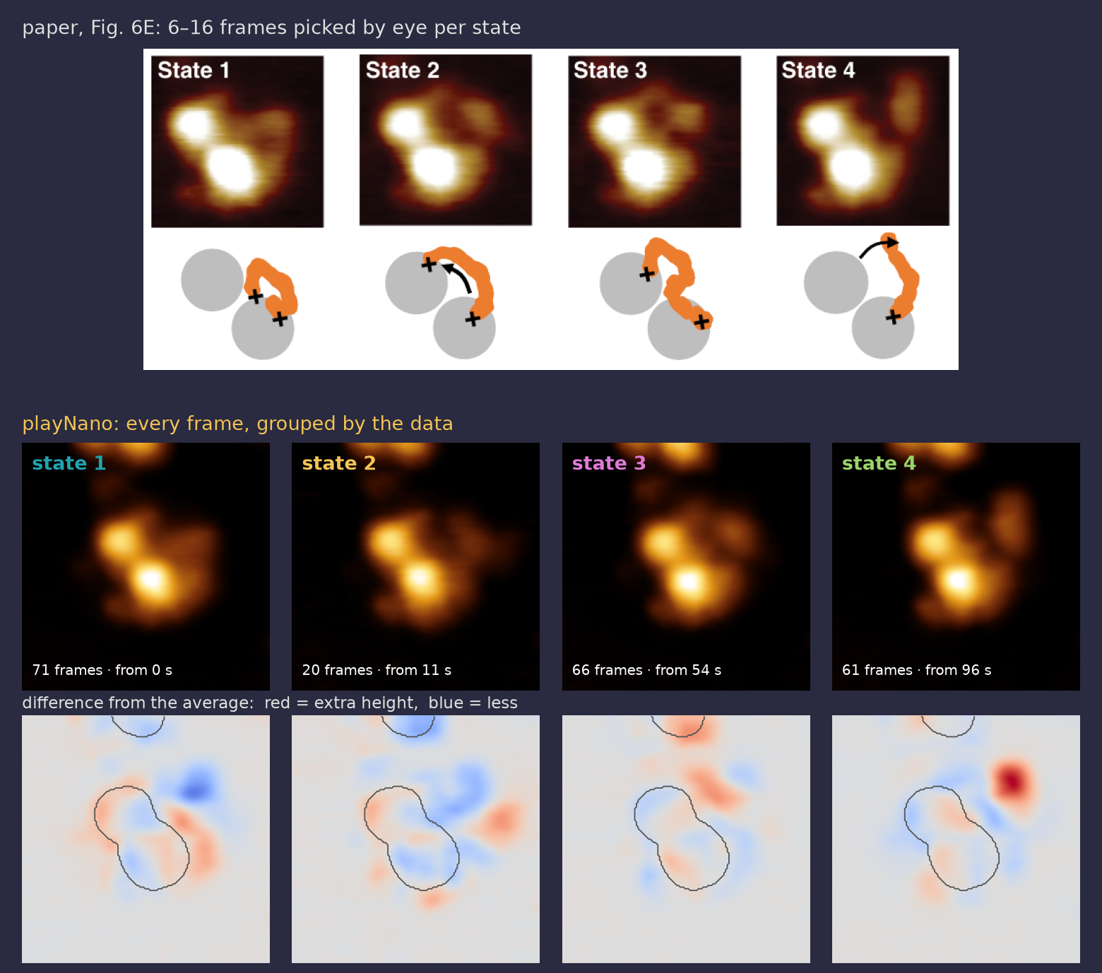
A DNA-repair protein reaching from one nucleosome to the next. The paper tracked it by eye. playNano reproduces that, then lets the movement itself pick out the states.
1 · Reproduce the paper: three points chosen by eye
Tracked and aligned: the box (inset) follows the particle, so p1–p3 stay on the same spot of the molecule
playNano: height under each pointPaper, Fig. 6D: the same three traces. p2 drops at 10–20 s; p3 rises from ~50 s, falls at ~100 s.
2 · Let the movement decide
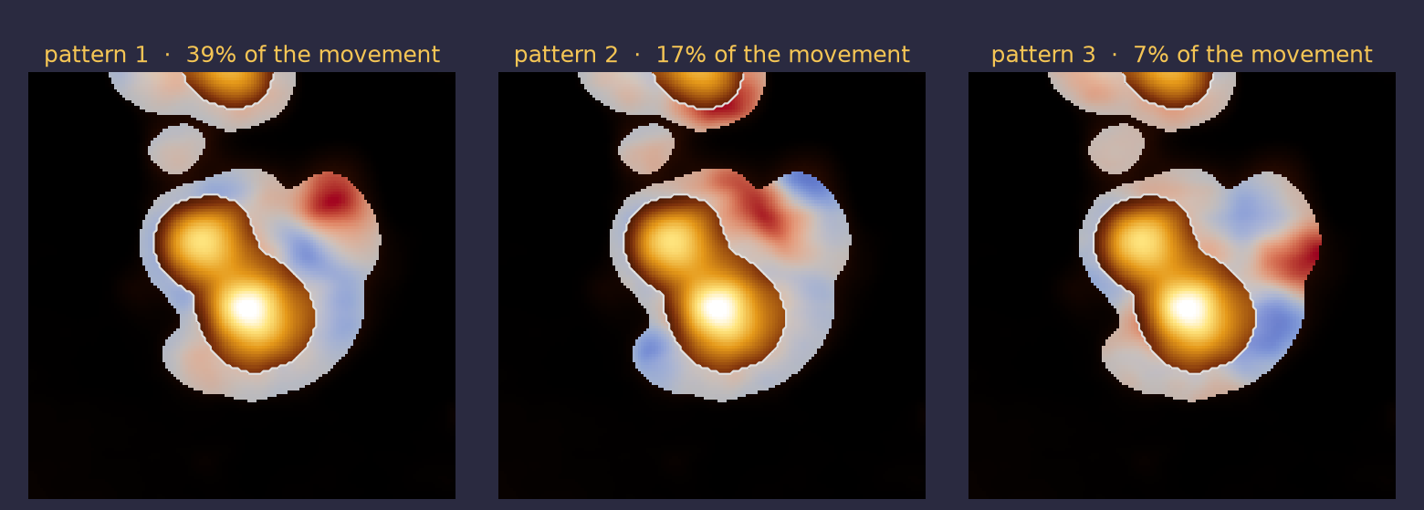
Subtract the average image and everything that stays still disappears; only what moves is left. Our eyes notice movement the same way. PCA then finds the main patterns of movement.
The three main patterns (nucleosomes masked). Red and blue swap: height appears in one place as it disappears in another.
3 · From movement to states
Every frame is a point: how much of pattern 1 and pattern 2 it contains. Frames that move alike land together.
1
Subtract the average
Only what moved in this frame is left.
2
Score each frame
How much of each pattern it contains: 5 numbers per frame. Each frame becomes a point.
3
Find the groups
Fit 2 to 8 groups (Gaussian mixture); BIC picks the number that explains the most without over-fitting. Each group is a state.
4
Use time
A state usually lasts more than one frame, so a hidden Markov model removes one-frame flickers (13 changes → 7).
Every frame labelled: frames that move the same way are grouped
When the state changes
54 s · 96 s
the two big changes, in all 45 settings I tried. Paper: bridging at 50–70 s, p3 drops at ~100 s
4–5
states, chosen by the data (BIC), not set in advance. Paper: "at least four"
Found without picking frames: states 3 and 4 line up with the paper's bridged and released forms, in look and in timing. Each average uses 20–71 frames.
playNano: load, level, track, alignPCA: patterns of movementGaussian mixture + BIC: how many stateshidden Markov model: no one-frame flicker
One molecule, one movie. Built in a marimo notebook on top of the recorded processing; next step: a plugin (see Plugins).
Antibody shape
unpublished · please don't photograph
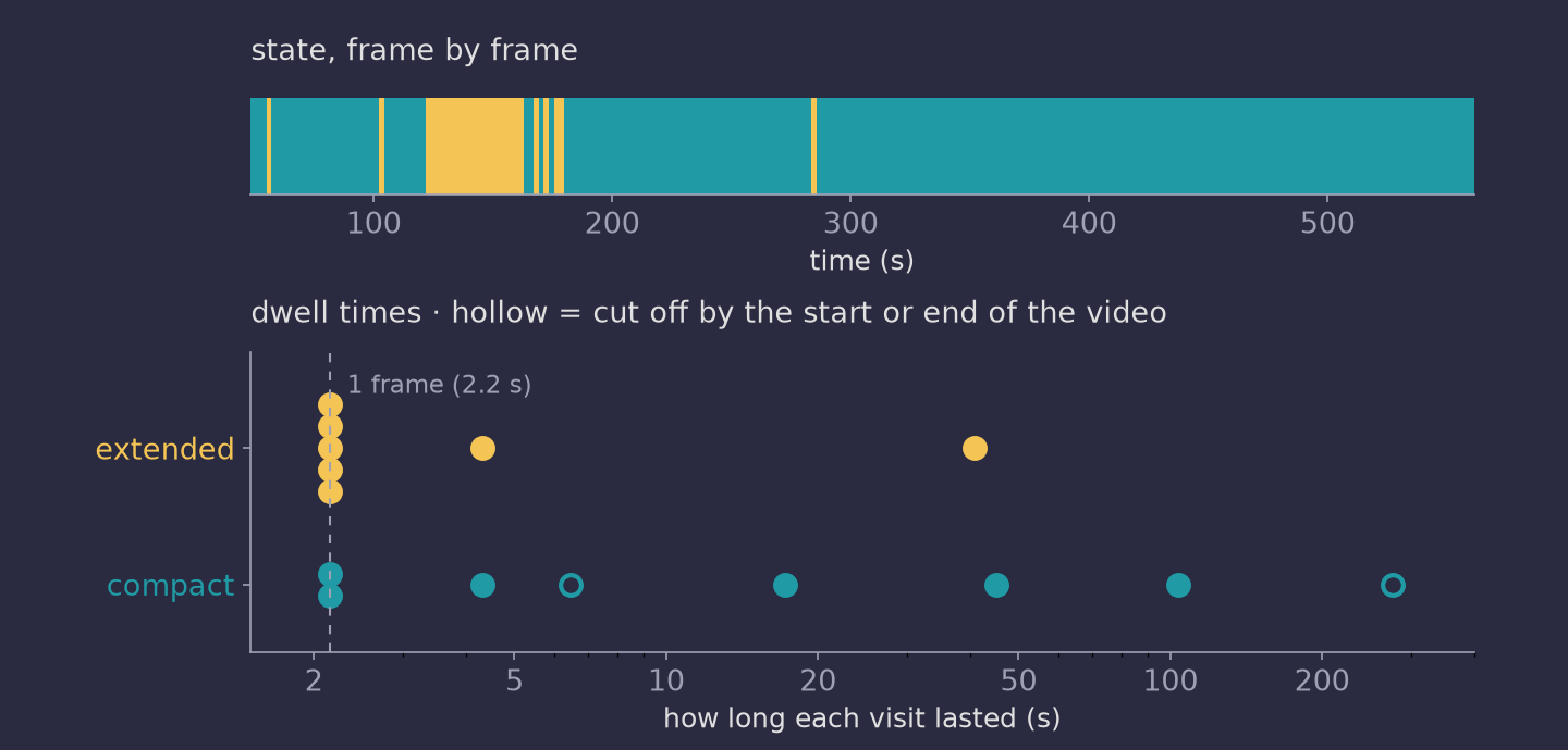
An antibody can sit compact or extended. Following one for 8.5 minutes: which is it, frame by frame?
Detected and tracked: green outline; box turns gold when extended
Following the particle
Largest dimension of the box, every frame; dashed line = threshold (38.7 nm, chosen by eye)
26 → 42 nm
typical compact → extended
11%
of frames extended
14
switches in 238 frames
2.2 s
per frame
How long does each state last?
Most extended visits last a single frame: faster switching than 2.2 s per frame can resolve. One long visit of 41 s.
Link objects frame to frame (≤ 80 px jump); keep the longest track
particle_boundary_size
Bounding box of the tracked mask → largest dimension
threshold=66 px
Parameter of the same step: each frame labelled compact or extended
Teal = built in, gold = my plugin (see Plugins). Run twice from the same recipe: identical results. A box depends on rotation; the true longest length (Feret) changes 1 frame of 238.
Raw
ML levelling (afMLevel plugin, twice) + smoothing, before any analysis
Plugins: your code as a recorded step
A recipe is a list of step names. playNano looks each name up among its own steps and every installed package, so a new step is just a package that registers a name.
Processing plugins
functions
playnano.filters
one frame in → one frame out
playnano.video_processing
whole video in → whole video out
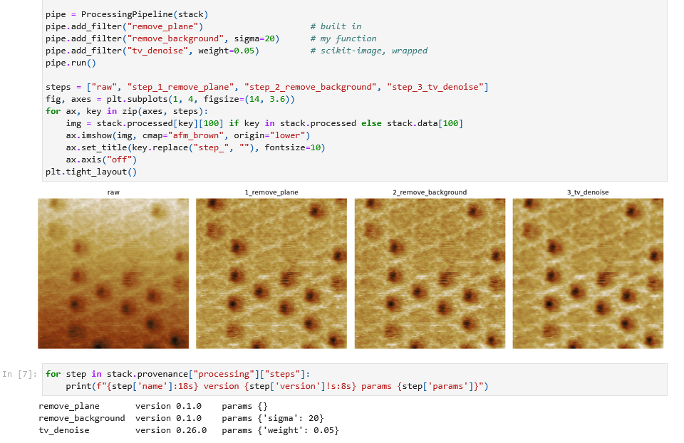
Your own filter, or a scikit-image one
Both live in your own small plugin package. You don't edit playNano or scikit-image.
pip install -e ./my_playnano_plugin, and both names work in any recipe.
Run in the demo notebook
tap to zoom
Built-in, my own and scikit-image steps in one pipeline; the record has scikit-image's version (0.26.0).
pyproject.tomlfilters.py
Already wrapped
afMLevel ML levelling · whole video or per framepnanolocz levelling · per frameTopoStats filters · per frame
Analysis modules
classes
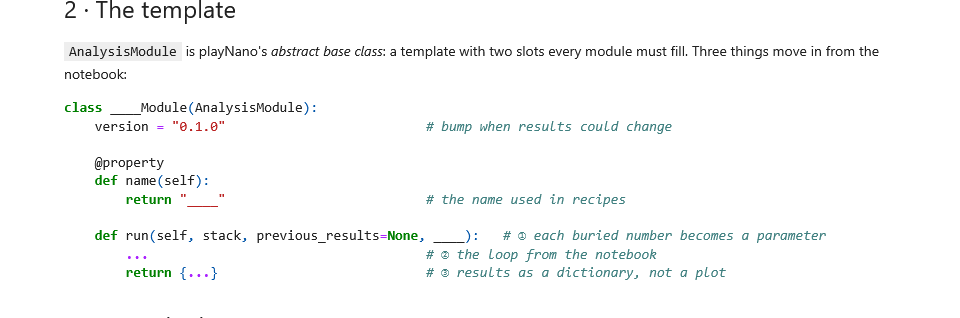
Built on playNano's abstract base class: a template that says what every module must have. Leave one out and Python won't create it.
class AnalysisModule(ABC):
@property
@abstractmethod
def name(self) -> str: ... # the name used in recipes
@abstractmethod
def run(self, stack, previous_results=None,
**params) -> dict: ... # results, saved + recorded
previous_results hands over earlier steps' outputs, e.g. the particle tracks.
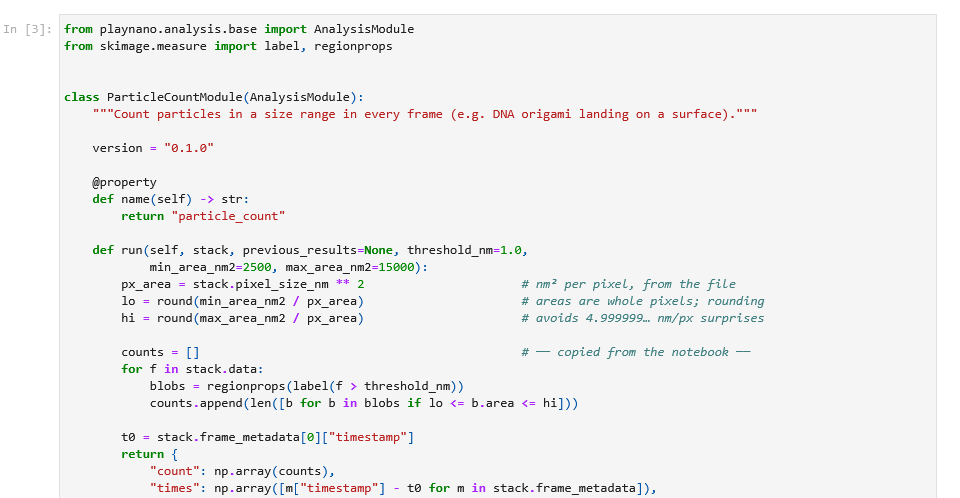
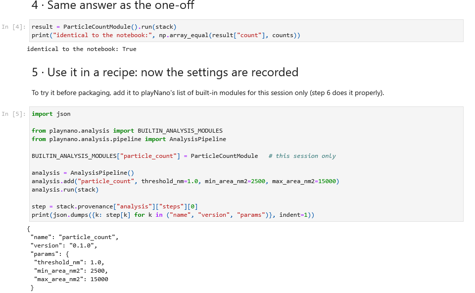
A one-off analysis becomes a shareable module
demo notebook · tap to zoom
1
One-off, in a project notebook
Counting origami triangles landing (public data). Works, but the settings are buried, sizes are in pixels, and the output is only a plot.
2
Copy the key parts into the template
The templateSettings → parameters; the loop copied as is
3
Same answer, and now it's recorded
4
Share it
One line in your package's pyproject.toml; anyone can then use it in a recipe.
My real one
particle_bounding.ipynb → particle_boundary_size in playNano-plugins, version 0.1.0: the antibody shape analysis.
Use it your way
Same recipe, same results, from a viewer, a script or the command line. Outputs open in the tools you already use.
playNano viewer
BRCA1–BARD1 on nucleosomes, NAR 2023
Raw → apply recipe → processed. Change the colour map and z-scale, then export GIF / MP4 / OME-TIFF / HDF5.
napari
OME-TIFF
Opens with the standard reader, at the right pixel size. Nothing added.
Fiji
Bio-Formats
Scale bar and time stamp drawn by Fiji from the file's own metadata: 0.39 nm/px, 0.655 s/frame.
Command line
playnano process video.h5-jpk \
--processing-file recipe.yaml \
--export tif,h5,npz --make-gif
playnano analyze out.h5 \
--analysis-file analysis.yaml# a whole experimentfor d in imaging-*/; do
playnano process "$d" --processing-file recipe.yaml --export tif
done
Batch: every video from one experiment, same recipe, one loop.
Python
from playnano.afm_stack import AFMImageStack
from playnano.processing.pipeline import ProcessingPipeline
stack = AFMImageStack.load_data("imaging.h5-jpk")
pipe = ProcessingPipeline(stack)
pipe.add_filter("remove_plane")
pipe.add_mask("mask_mean_offset", factor=0.6)
pipe.add_filter("gaussian_filter", sigma=0.8)
pipe.add_filter("align_frames")
record = pipe.run() # every step + parameter
The same steps can be saved as a YAML recipe and rerun from the command line.
Build the pipeline, run it, print the record, and plot the result in the notebook.
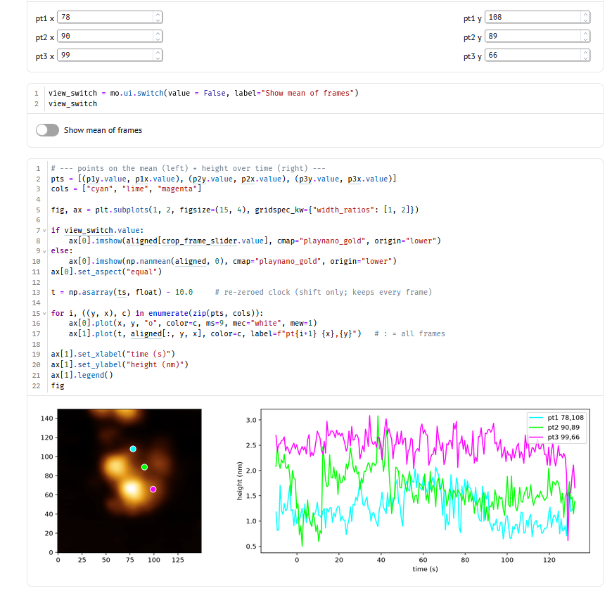
marimo
BRCA1–BARD1 analysis notebook
Reactive: move a point or flip the switch and the plots update. Height over time at three spots on the drift-corrected particle.
Colour maps are a measurement scale
If lightness doesn't rise evenly with height, low features vanish and HS-AFM videos flicker.
afm_brown
default
Linear lightness · R² 0.996
playnano_gold
high contrast
Full black → white · R² 0.978
classic_afm
legacy look
Dark plateau hides the substrate · R² 0.763
afmhot
matplotlib
Kinked lightness · R² 0.872
Same published video (BRCA1–BARD1, NAR 2023), with the height range re-fitted every frame as auto-scaling does. Watch the background.
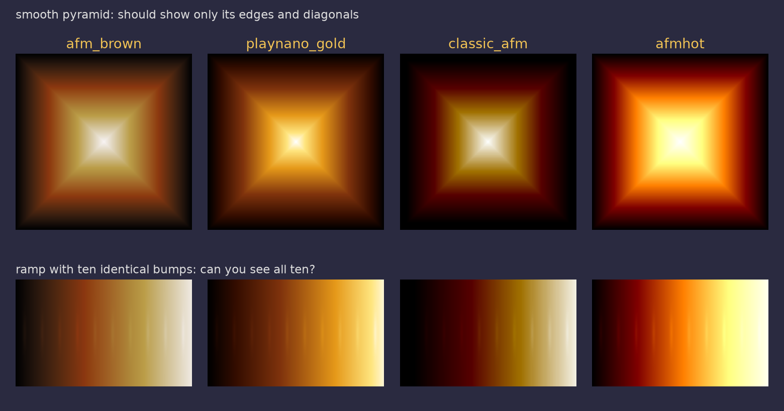
Test patterns
idea from ehtplot (Event Horizon Telescope)
A bent lightness curve invents features and hides others. classic_afm draws a dark ring and a bright square that aren't in the data, and loses the bumps in its dark third; afmhot loses them at the bright end.
Why I made new ones
Equal steps in height should look like equal steps in brightness. The familiar AFM browns bend: a long black stretch at the bottom, then a jump.
import playnano # registers them
plt.imshow(h, cmap="afm_brown")
Ordinary matplotlib colour maps: use them in any script, or in napari and Fiji via exports.
Perceived lightness (CIE L*) along each map. Dashed straight line = perfectly linear.
Inspired by the colour-map work in ehtplot (github.com/liamedeiros/ehtplot): "a poorly chosen colormap … can fool the human eyes".